

This post assumes you already know the basic quicksort algorithm, asymptotic notation, and how to read simple probability and expectation arguments. If those are new, a quick refresher on deterministic quicksort and expected value will make the proofs here much easier to follow.
The Algorithm#
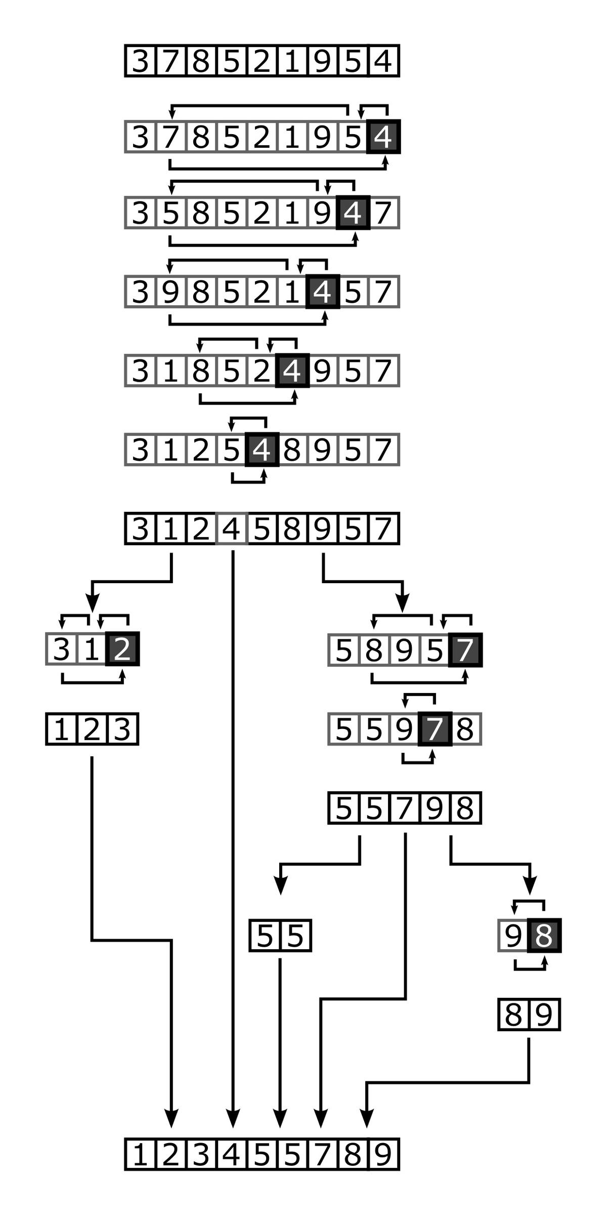
Randomized quicksort is just quicksort where the pivot is chosen uniformly at random from the current subarray. The randomness can be explicit (pick a random index) or implicit (shuffle the array first and use the first element as pivot). The algorithm is the same either way.
R-QUICKSORT(A):
  if |A| <= 1: return A
  choose pivot p uniformly at random from A
  partition A into L = {x < p}, E = {x = p}, G = {x > p}
  return R-QUICKSORT(L) + E + R-QUICKSORT(G)
We only need to analyze the number of comparisons, since partitioning dominates the runtime. The deterministic worst case is still \( O(n^2) \), but randomization makes the expected cost \( O(n \log n) \) and makes the exact maximum-comparison path factorially unlikely.
The equality bucket handles duplicate keys in the algorithm. For the comparison-count proof below, I use the standard distinct-keys model.
Complexity Analysis through the Expected Number of Comparisons#
Assume all keys are distinct, and label them in sorted order as \( z_1 < z_2 < \dots < z_n \). Let \( X_{ij} \) be the indicator variable for whether \( z_i \) and \( z_j \) are ever compared (for \( i < j \)).
The total number of comparisons is
$$ C = \sum_{1 \le i < j \le n} X_{ij}. $$So by linearity of expectation,
$$ \mathbb{E}[C] = \sum_{1 \le i < j \le n} \mathbb{E}[X_{ij}] = \sum_{1 \le i < j \le n} \Pr[X_{ij} = 1]. $$Key claim. \( z_i \) and \( z_j \) are compared iff the first pivot chosen from the set \( {z_i, z_{i+1}, \dots, z_j} \) is either \( z_i \) or \( z_j \).
Proof. Consider the first pivot chosen from that contiguous block in sorted order. If the pivot is some \( z_k \) with \( i < k < j \), then \( z_i \) and \( z_j \) fall into different partitions and are never compared. If the first pivot is \( z_i \) (or \( z_j \)), then during that partition step, \( z_i \) (or \( z_j \)) is compared against every element in the block, including \( z_j \) (or \( z_i \)). QED.
Since the pivot is chosen uniformly among the \(j - i + 1\) elements in the block,
$$ \Pr[X_{ij} = 1] = \frac{2}{j - i + 1}. $$Therefore
$$ \mathbb{E}[C] = \sum_{1 \le i < j \le n} \frac{2}{j - i + 1}. $$Let \( k = j - i + 1 \). For each fixed \( k \), there are \( n - k + 1 \) pairs with that distance, so
$$ \mathbb{E}[C] = \sum_{k=2}^{n} (n - k + 1) \cdot \frac{2}{k} = 2 \sum_{k=2}^{n} \frac{n - k + 1}{k}. $$Using \( \sum_{k=1}^{n} \frac{1}{k} = H_n \) (the \( n \)-th harmonic number), we get
$$ \mathbb{E}[C] = 2(n+1)H_n - 4n = O(n \log n). $$This is a full, exact expectation result. No recurrence solving needed.
How Unlikely Is the Exact Worst Case?#
The exact maximum-comparison path happens when every pivot is an extreme element: either the minimum or maximum of its current subarray. For an input of size \( n \), this path has probability
$$ \Pr[\text{worst case}] = \prod_{k=2}^{n} \frac{2}{k} = \frac{2^{n-1}}{n!}, $$which is factorially small. For perspective, when \( n = 10 \) this is \( 2^9/10! \approx 0.0141\% \), and when \( n = 20 \) it’s \( 2^{19}/20! \approx 0.0000000000216\% \). The algorithm keeps its worst-case bound, but randomization pushes the maximum-comparison path into the far tail.
Why \(O(n \log n)\) Happens with High Probability#
Call a pivot good if both recursive subproblems have size at most \( 3/4 \) of the current subproblem. After \( t \) good pivots on any fixed element’s recursive path, the subproblem containing that element has size at most \( (3/4)^t n \). We want this to be \( \le 1 \), so the recursion ends. This requires \( t \ge c_0 \log n \) for some constant \( c_0 \).
Each pivot is good with probability at least \( 1/2 \) (any pivot from the middle half works), and this lower bound holds regardless of what happened before. Consider the recursive path followed by one fixed element. Let \( G \) be the number of good pivots in the first \( m \) pivot choices on that path. Although these events are not independent, each pivot is good with conditional probability at least \( 1/2 \), so \( G \) stochastically dominates a \( \text{Binomial}(m, 1/2) \) random variable.
Choose \( m = \frac{2c_0}{1 - \delta} \log n \) for some fixed \( \delta \in (0,1) \). Then the mean is \( \mu = m/2 = \frac{c_0}{1 - \delta} \log n \), and the bad event (insufficient progress) is \( G < c_0 \log n = (1 - \delta)\mu \). By a standard Chernoff bound for a binomial,
$$ \Pr[G < (1 - \delta)\mu] \le \exp\left(-\frac{\delta^2 \mu}{2}\right). $$So
$$ \Pr[G < c_0 \log n] \le \exp\left(-\frac{\delta^2 \mu}{2}\right) = n^{-\frac{\delta^2}{2(1 - \delta)}c_0}. $$For a fixed element, the probability that it is still in a nontrivial subproblem after \( m = \Theta(\log n) \) recursive calls is polynomially small. Choose constants \( \delta \) and \( c_0 \) so that the exponent is at least 2, giving probability at most \( n^{-2} \). By a union bound over all \( n \) elements, the probability that any element has recursion depth greater than \( m \) is at most \( O(n) \) times this quantity.
$$ \Pr[\text{any element's path takes too long}] \le O(n) \cdot n^{-2} = O(n^{-1}), $$which goes to 0 as \( n \to \infty \). Since each recursion level partitions disjoint subarrays whose total size is at most \( n \), an \( O(\log n) \) recursion depth implies \( O(n \log n) \) total partitioning work with high probability.
Intuitively, this is no different from repeatedly tossing a fair coin. For example, in 40 tosses we expect 20 heads on average, and the probability of seeing fewer than 10 heads is only about 0.03%. Any large deviation from the expectation is extremely unlikely. Likewise, the probability that randomized quicksort fails to make sufficient progress after \( \Theta(\log n) \) steps decays polynomially in \( n \), with an exponent that grows linearly in \( c_0 \).
Summary#
Randomization makes quicksort efficient in expectation without changing its basic structure. The result is a \( O(n \log n) \) expected runtime algorithm, and the probability of significantly deeper recursion decays as \( n^{-\Theta(1)} \).
References#
- Rajeev Motwani and Prabhakar Raghavan, Randomized Algorithms, Cambridge University Press, 1995, Chapter 1.